Analytic solutions for height and velocity profile.

This section demonstrates how to use the Depth_result class which allows to calculate the depth and velocity profile of the flow at a given time.

To simplify the calculations, only 1D models will be taken into account. Under the assumptions of one-dimensional flow and an incompressible fluid, it is possible to model the flow using the Saint-Venant equations, which form a system of partial differential equations derived from the principles of mass conservation (continuity equation) and momentum conservation (momentum equation). In a case of a flat surface, the Saint-Venant’s system can be expressed as:

\[\begin{split}\begin{cases} \partial_t h + \partial_x (hu) = 0 \\\\ \partial_t (hu) + \partial_x (\alpha hu^2) + \partial_x (\frac{1}{2}kgh^2 \cos{\theta}) = gh\sin{\theta} - S \end{cases}\end{split}\]

where

• \(h\): fluid depth.

• \(u\): fluid velocity.

• \(g\): gravitational acceleration.

• \(\alpha\): form factor associated with nonlinear velocity profiles.

• \(k\): coefficient introduced to take into account internal friction.

• \(\partial_t\): partial derivative with respect to time.

• \(\partial_x\): partial derivative with respect to space.

• \(\theta\): slope of the surface.

• \(S\): source term integrating the dissipative effects of energy which slows the flow.

In the most common cases, \(\alpha = 1\) and \(k = 1\), which leads to the following equations which will be reused subsequently:

\[\begin{split}\begin{cases} \partial_t h + \partial_x (hu) = 0 \\\\ \partial_t (hu) + \partial_x (hu^2) + \frac{1}{2}g\cos{\theta} \partial_x (h^2) = gh\sin{\theta} - S \end{cases}\end{split}\]

As already said, the source term \(S\) contains all dissipative effects of energy which slows the flow (due to friction or viscosity). A large number of models exist to express this term as a function of flow conditions.

For example, we can cite the general formulation for a Coulomb-type friction law:

\[S = h \mu \left( g \cos{\theta} + \gamma u^2 \right)\]

where \(\gamma = \frac{1}{R}\), \(R\) being the radius of curvature, \(\theta\) the surface slope and \(\mu\) the coefficient of basal friction. The coefficient of friction \(\mu\) has multiple expressions, it can be either a constant or a function of \(h\) and \(u\).

We can also cite an equation combining the Darcy-Weisbach and Manning laws for hydraulic models:

\[S = g n^2 \frac{u^2}{h^{1/3}}\]

where \(n\) is Manning coefficient (in \(s.m^{-1/3}\)).

For viscoplastic models, it is possible to use the Herschel-Bulkley formula:

\[S = \frac{\tau_y}{\rho} \left[ 1 + 1.93 \left( \frac{\tau_y}{k} \left( \frac{h}{u} \right)^{1/3} \right)^{-0.9} \right]\]

Or Bingham fomrula:

\[S = \frac{3}{2} \frac{\tau_y}{\rho} + 3 \frac{\nu u}{\rho h}\]

where \(\tau_y\) and \(\rho\) are the yield stress and the density, \(\nu\) the dynamic viscosity and \(k\) consistency factor.

Finally for empiric models, we can use Voellmy’s formula:

\[S = h \mu \left( g \cos{\theta} + \gamma u^2 \right) + \frac{u^2}{\xi}\]

with \(\gamma = \frac{1}{R}\), \(R\) being the radius of curvature, \(\theta\) the surface slope, \(\mu\) the coefficient of basal friction and \(\xi\) an empirical parameter called the turbulence coefficient.

---

References

Peruzzetto, M., Grandjean, G., Mangeney, A., Levy, C., Thiery, Y., Vittecoq, B., Bouchut, F., Fontaine, F.R., & Komorowski, J.-C., 2023, Simulation des écoulements gravitaires avec les modèles d’écoulement en couche mince : état de l’art et exemple d’application aux coulées de débris de la Rivière du Prêcheur (Martinique, Petites Antilles), Revue Française de Géotechnique, vol. 176, p. 1, doi:10.1051/geotech/2023020.

Savage, S.B., & Hutter, K., 1991, The dynamics of avalanches of granular materials from initiation to runout. Part I: Analysis, Acta Mechanica, v. 86(1), p. 201–223.

Dam-break problem

Below are grouped several analytical solutions for a dam-break problem under conditions varying from one model to another. The next table will summarize the main differences between the models:

Feature	Ritter	Stocker	Mangeney	Dressler	Chanson
Domain	Dry bed	Wet bed	Dry bed	Dry bed	Dry bed
Friction Modeling	Ignored	Ignored	With friction angle \(\delta\)	With Chézy coefficient \(C\)	With Darcy friction coefficient \(f\)
Bed Slope	Only horizontal	Only horizontal	Inclined	Only horizontal	Only horizontal
Initial Fluid Height	\(h_0 > 0\)	\(h_0 > 0\)	\(h_0 > 0\)	\(h_0 > 0\)	\(h_0 > 0\)
Domain Height If Wet	\(0\)	\(0 < h_r < h_0\)	\(0\)	\(0\)	\(0\)
Initial Velocity	\(u(x,0) = 0\)	\(u(x,0) = 0\)	\(u(x,0) = 0\)	\(u(x,0) = 0\)	\(u(x,0) = 0\)
Solution Zones	3 (reservoir, rarefaction, dry)	4 (reservoir, rarefaction, shock, wet)	3 (reservoir, rarefaction, dry)	4 (reservoir, rarefaction, tip, dry)	4 (reservoir, rarefaction, tip, dry)
Shock Wave	None	Yes	None	None	None
Wave Speeds	Closed-form	Via \(c_m\)	Closed-form	Via \(c_m\)	Via \(U(t)\)
Initial water volume	Finite	Finite	Infinite	Finite	Finite
Reference	Ritter (1892)	Stocker (1957)	Mangeney et al. (2000)	Dressler (1952)	Chanson (2005)

Below is a gallery of functions for each model type illustrating their specificity and how they work:

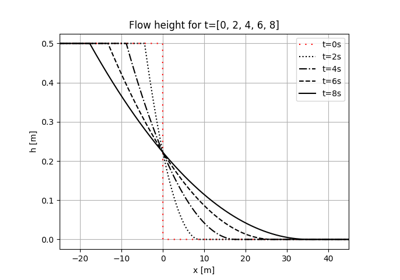
Analytical solution of a dam-break problem on a dry slope with friction (Chanson)

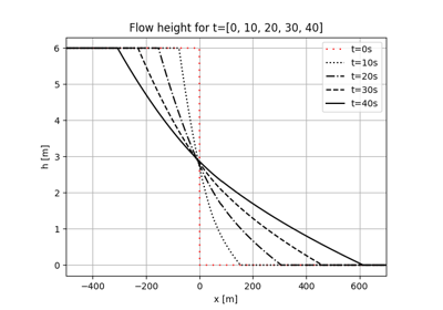
Analytical solution of a dam-break problem on a dry slope with friction (Chanson)

Analytical solution of a dam-break problem on a dry slope with friction (Dressler)

Analytical solution of a dam-break problem on a dry slope with friction (Dressler)

Analytical solution of a dam-break problem on a dry slope with friction (Mangeney et al.)

Analytical solution of a dam-break problem on a dry slope with friction (Mangeney et al.)

Analytical solution of a dam-break problem on a dry bed without friction (Ritter)

Analytical solution of a dam-break problem on a dry bed without friction (Ritter)

Analytical solution of a dam-break problem on a wet bed without friction (Stocker)

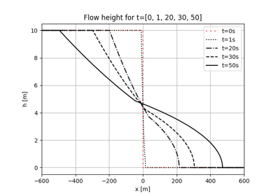
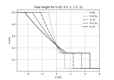
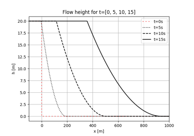
Analytical solution of a dam-break problem on a wet bed without friction (Stocker)