Combine multiple simulation results

We show here how multiple simulation results can be combined to build, e.g., scenario-based hazard maps.

Initial import

import matplotlib.pyplot as plt
import numpy as np

import tilupy.read
import pytopomap.plot

Specify where results are stored. If results are stored in a different folder than ‘./shaltop_frankslide’, folder_simus must be changed accordingly

# import tilupy.download_data
# tilupy.download_data.import_shaltop_frankslide()
folder_simus = "./shaltop_frankslide"

We consider here three simulations with the Coulomb rheology and friction coefficients \(\mu_S=\tan(\delta)\), with \(\delta=15°\), \(\delta=20°\) and \(\delta=25°\). The lower the friction angle \(\delta\), the higher the mobility. We will thus create map combining the impacted area for the three friction coefficients. We first make a list with the different parameters files

deltas = [15, 20, 25]
param_files = [
    "delta_{:5.2f}".format(delta).replace(".", "p") + ".txt" for delta in deltas
]

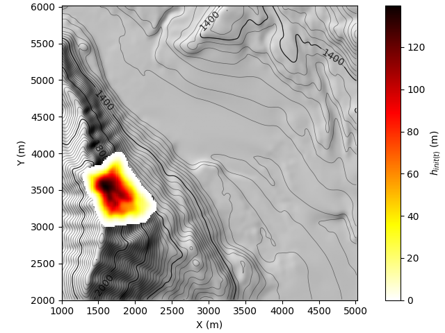
Initiate result array with the same shape as the grid in the simulations. We also display the initial mass.

res = tilupy.read.get_results(
    "shaltop", folder=folder_simus, file_params=param_files[0]
)
impacted_area = np.zeros(res.z.shape)
res.plot("h_init")

[WARNING] h_init not found with _read_from_file for shaltop, use get_spatial_stat

<Axes: xlabel='X (m)', ylabel='Y (m)'>

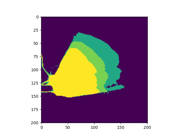
For each simulation, we recover the total impacted area by considering the area where the mximum simulated thickness is aboce a given threshold, here h_thresh=0.1. It is added incrementally to the array impacted_area, starting with the most mobile simulation (\(\delta=15°\)).

h_thresh = 0.1
for i in range(3):
    tmp = tilupy.read.get_results(
        "shaltop", folder=folder_simus, file_params=param_files[i]
    )
    ind = (
        tmp.h_max > h_thresh
    )  # here res.h_max is equivalent to res.get_output('h_max').d
    impacted_area[ind] = deltas[i]
plt.imshow(impacted_area)

<matplotlib.image.AxesImage object at 0x74149667d1d0>

We assume that increasing the friction cofficient necessarily reduces the impacted area. In the array impacted_area

• impacted_area=25 for a point impacted in the three simulations

• impacted_area=20 for a point impacted with \(\delta=20°\) and \(\delta=15°\)

• impacted_area=15 for a point impacted with \(\delta=15°\) only

• impacted_area=0 for a point impacted by no simulation

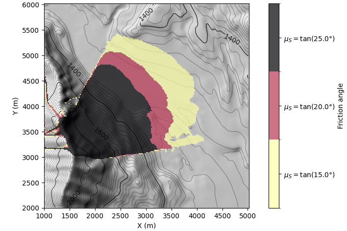
Results are rendered with pytopomap.

axe = pytopomap.plot.plot_data_on_topo(
    res.x,
    res.y,
    res.z,
    impacted_area,
    figsize=(18 / 2.54, 12 / 2.54),
    cmap="inferno_r",
    unique_values=True,  # Make nice colorbar considering unique values
    alpha=0.7,  # Add transparency to see the topography
    plot_colorbar=True,
    colorbar_kwargs=dict(label="Friction angle"),
)
labels = ["$\\mu_S=\\tan({:.1f}$°$)$".format(delta) for delta in deltas]
axe.figure.axes[-1].set_yticklabels(labels)

[Text(1, 16.0, '$\\mu_S=\\tan(15.0$°$)$'), Text(1, 20.0, '$\\mu_S=\\tan(20.0$°$)$'), Text(1, 24.0, '$\\mu_S=\\tan(25.0$°$)$')]