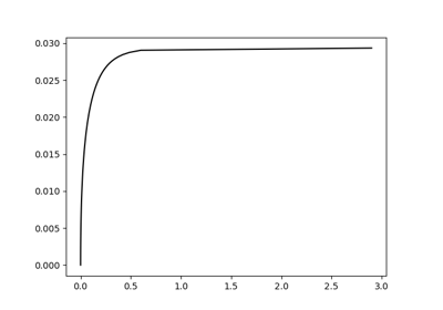
Analytic solutions for the morphology of the final state of the front.
This section demonstrates how to use the Shape_result class which allows to compute the shape of the flow front at the final step of the flow.
Coussot’s model
Coussot et al proposed a formula in 1996 to approximate the geometry of the frontal lobe of a flow at a final instant for rheological test on an inclined surface:
with \(D\) and \(H\) being the normalized version of the distance of the front \(d\) and the fluid depth \(h\), obtained by computing:
where
\(h\): fluid depth.
\(x\): spatial dimension.
\(g\): gravitational acceleration.
\(\rho\): fluid density.
\(\tau_c\): threshold constraint.
\(\theta\): slope of the surface.
In a case where \(\theta = 0\), the equations are slightly different:
with:
References
Coussot, P., Proust, S., & Ancey, C., 1996, Rheological interpretation of deposits of yield stress fluids, Journal of Non-Newtonian Fluid Mechanics, v. 66(1), p. 55–70, doi:10.1016/0377-0257(96)01474-7.