Coussot’s model example

This example demonstrates the final shape of simulated flow using Coussot’s equation.

The frontal lobe shape of the simulated flow at the final step is given by

\[D = - H - \ln(1 - H)\]

where

• \(H\): normalized fluid depth.

• \(D\): normalized distance of the front from the origin.

\(H\) and \(D\) are obtained with these expressions:

\[D = \frac{\rho g d (\sin(\theta))^2}{\tau_c \cos(\theta)} \text{ and } H = \frac{\rho g h \sin(\theta)}{\tau_c}\]

with:

• \(h\): fluid depth.

• \(d\): distance of the front from the origin.

• \(g\): gravitational acceleration.

• \(\rho\): fluid density.

• \(\tau_c\): threshold constraint.

• \(\theta\): slope of the surface.

Implementation

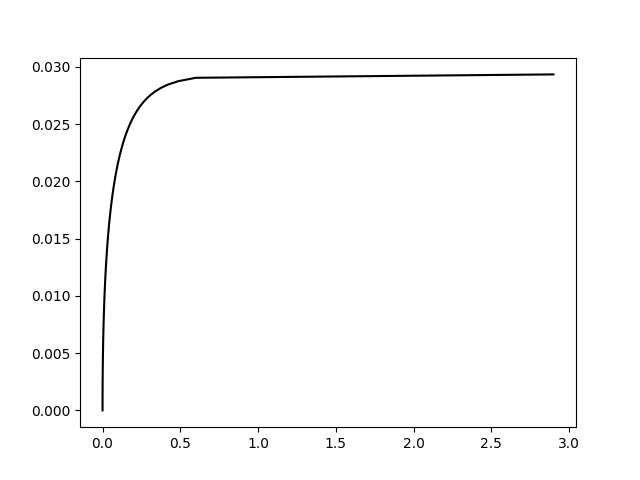
First import required packages and define the context. For this example we will use a fluid with a density of \(\rho = 1000 kg/m^3\): and \(\tau_c = 50 Pa\), with a slope of \(\theta = 10°\):

from tilupy.analytic_sol import Coussot_shape
import matplotlib.pyplot as plt

case_1 = Coussot_shape(rho=1000, tau=50, theta=10)
case_1.compute_rheological_test_front_morpho()
plt.plot(case_1.d, case_1.h, color="black")
plt.show()

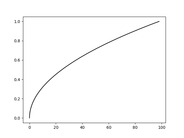
If \(\theta = 0°\), the equations are slightly different:

\[D^* = \frac{{H^*}^2}{2}\]

with:

\[D^* = \frac{\rho g d}{\tau_c} \text{ and } H^* = \frac{\rho g h}{\tau_c}\]

case_2 = Coussot_shape(rho=1000, tau=50, theta=0, h_final=1)
case_2.compute_rheological_test_front_morpho()
plt.plot(case_2.d, case_2.h, color="black")
plt.show()

Original reference:

Coussot, P., Proust, S., & Ancey, C., 1996, Rheological interpretation of deposits of yield stress fluids, Journal of Non-Newtonian Fluid Mechanics, v. 66(1), p. 55-70, doi:10.1016/0377-0257(96)01474-7.