Calibration example

We show here how multiple simulations can be processed at once to compare simulations to observed data. In this example, observations consist in an impacted area and a travel distance along a given profile.

Initial imports. We use here the geopandas package to load and process observation data. geopandas is not installed along with tilupy, and must be installed separately to run this example. tilupy bult-in calibration functions use only shapely.

import os
import tilupy.read
import tilupy.calibration
import tilupy.raster
import geopandas as gpd
import matplotlib.pyplot as plt

Download simulation data and pseudo-observation data. The calibration folder contains a ascii raster with an hypothecial observed impacted area (extent_example.asc), a shapefile with the profile along which travel distance must be measured (profile.shp) and a shapefile with the point giving the observed front position along this profile (front_position.shp).

Note that all objects share the same metric projection system, but their position is completely arbitrary.

# Un comment the first line to dowload the data
# tilupy.download_data.import_shaltop_frankslide()
folder_simus = "./shaltop_frankslide"
x, y, obs_extent = tilupy.raster.read_ascii(
    os.path.join(folder_simus, "calibration", "extent_example.asc")
)
file_profile = os.path.join(folder_simus, "calibration", "profile.shp")
profile = gpd.read_file(file_profile)
file_front = os.path.join(folder_simus, "calibration", "front_position.shp")
front = gpd.read_file(file_front)

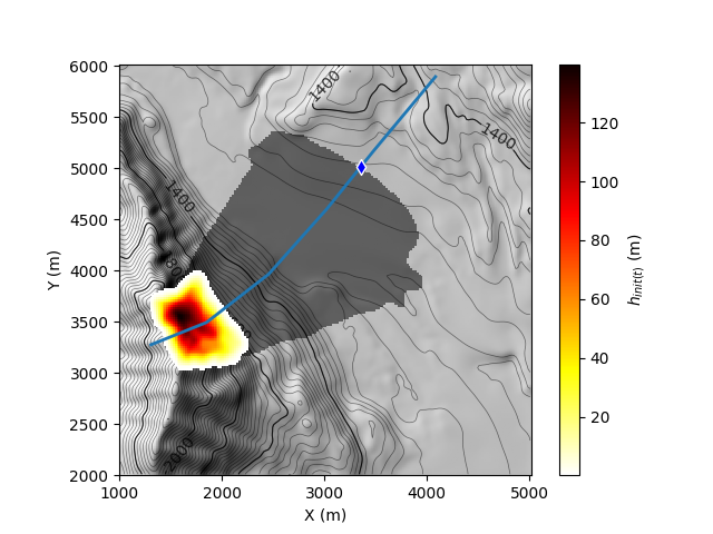
Visualize the topography, the initial mass and the “observed” impacted area (light black), the profile (blue line) and the observed front position (diamond)

res = tilupy.read.get_results(
    "shaltop", folder=folder_simus, file_params="delta_25p00.txt"
)
x, y, z = res.x, res.y, res.z
gif, axe = plt.subplots()
res.plot("h_init", ax=axe, mask=obs_extent, alpha_mask=0.5, vmin=0.1)
profile.plot(ax=axe, lw=2, zorder=4)
front.plot(
    ax=axe, marker="d", markersize=50, edgecolor="white", facecolor="b", zorder=5
)

[WARNING] h_init not found with _read_from_file for shaltop, use get_spatial_stat

<Axes: xlabel='X (m)', ylabel='Y (m)'>

Simulations were carried out in shaltop with the Coulomb rheology, with with, \(\delta=10°\), \(\delta=15°\), \(\delta=20°\) and \(\delta=25°\). For the sake of the example, the synthetic observations correspond to the area where the maximum simulated thickness is above 5m with \(\delta=15°\).

We compare the travel distance and the extent between observations and simulations with different thickness thresholds: 0.5m, 1m, 2.5m, 5m, 10m and 20m. The difference between the “observed” and simulated extent is quatified with the CSI (Critical Success Index), defined as:

\[CSI = \frac{TP}{TP+FP+FN}\]

where \(TP\) is the number of true positives (cells where the landslide is simulated and observed), \(FP\) is the number of false positives (cells where the landslide is simulated and not observed) and \(FN\) is the number of false negatives (cells where the landslide is not simulated but observed).

# Thickness thresholds used for extent determination in simulations
h_threshs = [0.5, 1, 2.5, 5, 10, 20]
# methods for calibration
methods = ["CSI", "diff_runout"]
# friction coefficients tested in simulations and associated parameter files
deltas = [10, 15, 20, 25]
parameter_files = [
    "delta_{:05.2f}".format(delta).replace(".", "p") + ".txt" for delta in deltas
]

Construct list of simulations used for calibration

simus = [
    tilupy.read.get_results("shaltop", folder=folder_simus, file_params=file)
    for file in parameter_files
]

Parameters used for computing the CSI and the runout difference, and definition of parameters associated to each simulation (correspond to a parameters read in the input parameter files). Here we consider only on parameter, but multiple parameter can be recorded if necessary.

kws_csi = dict(
    observation=obs_extent,  # array with the extent to be matched
    state="h_max",  # result used to estimate this extent in simulation
)
# Get hapely geometries associated to the geodataframes for the front
# and the profile, and use them to compute the runout difference.
front_point = front.geometry.iloc[0]
profile_line = profile.geometry.iloc[0]
kws_diff_runout = dict(
    point=front_point,  # Position of the observed front
    section=profile_line,  # Profile used to determine the front position in simulation
    state="h_max",  # result used to estimate the front poition in simulation, along the profile
    orientation="S-N",  # Prefered orientation of the profile (here South-North)
)
recorded_params = ["delta1"]

Estimate calibration results. it is provided as a pandas dataframe with one line per simulation.

calib_res = tilupy.calibration.eval_simus(
    simus,
    methods,  # Here, ['CSI', 'diff_runout']
    h_threshs,
    [kws_csi, kws_diff_runout],
    recorded_params=recorded_params,
)
calib_res.head()

	delta1	CSI	diff_runout	h_threshs
0	10.0	0.552184	935.36214	0.5
1	10.0	0.578586	935.36214	1
2	10.0	0.615562	935.36214	2.5
3	10.0	0.666052	935.36214	5
4	10.0	0.673238	935.36214	10

You can also define the input simus as a pandas DataFrame (or a dict) with keys (or column names) corresponding to the name of input parameters of tilupy.read.get_results(), and providing associated values. The model name must then be provided to :func:eval_simus that will automatically load results. The values specified in the original simus dict or DataFrame are then passed on to the result of eval_simus(). In this case example, for instance:

simus = dict(folder=[folder_simus] * len(parameter_files), file_params=parameter_files)
calib_res = tilupy.calibration.eval_simus(
    simus,
    methods,  # Here, ['CSI', 'diff_runout']
    h_threshs,
    [kws_csi, kws_diff_runout],
    recorded_params=recorded_params,
    model_name="shaltop",
)
calib_res.head()

	folder	file_params	delta1	CSI	diff_runout	h_threshs
0	./shaltop_frankslide	delta_10p00.txt	10.0	0.552184	935.36214	0.5
1	./shaltop_frankslide	delta_10p00.txt	10.0	0.578586	935.36214	1
2	./shaltop_frankslide	delta_10p00.txt	10.0	0.615562	935.36214	2.5
3	./shaltop_frankslide	delta_10p00.txt	10.0	0.666052	935.36214	5
4	./shaltop_frankslide	delta_10p00.txt	10.0	0.673238	935.36214	10

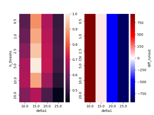
Results can be plotted as heatmaps.

tilupy.plot.plot_heatmaps(
    calib_res,
    ["CSI", "diff_runout"],
    "h_threshs",
    "delta1",
)

<Figure size 640x480 with 4 Axes>

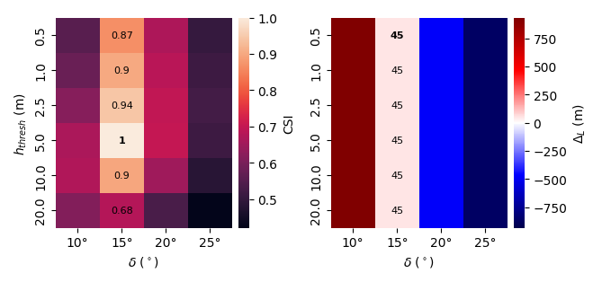
Plot can be customized. The best calibration values for each threshold can be identified following a method given in best_values. It will be highlighted with a point (plot_best_value='point') or written (plot_best_value='point'). The labels correspond to the data_frame columns but can be changed following the labels dict. You can also customize the heatmap with kwargs passed to seaborn.heatmap.

best_values = dict(CSI="max", diff_runout="min_abs")
labels = dict(
    h_threshs="$h_{thresh}$ (m)",
    delta1="$\delta$ ($^\circ$)",
    diff_runout="$\Delta_L$ (m)",
)
heatmap_kws = dict(xticklabels=["10°", "15°", "20°", "25°"])
fig = tilupy.plot.plot_heatmaps(
    calib_res,
    ["CSI", "diff_runout"],
    "h_threshs",
    "delta1",
    figsize=(17 / 2.54, 8 / 2.54),
    best_values=best_values,
    aggfunc="mean",
    notations=labels,
    heatmap_kws=heatmap_kws,
    plot_best_value="text",
)
fig.tight_layout()