Load and display results as maps

We show here how simulation results can be loaded, and 2D results displayed as figures.

Initial import

import matplotlib.pyplot as plt
import tilupy.read

Import pytopomap package to control pricesly plots. pytopomap is used by tilupy to generate plots (see below)

import pytopomap.plot

Initatiate Results instance. The first two lines can be used to download examples of results. If results are stored in a different folder than ‘./shaltop_frankslide’, folder_simus must be changed accordingly

# import tilupy.download_data
# tilupy.download_data.import_shaltop_frankslide()
folder_simus = "./shaltop_frankslide"
res = tilupy.read.get_results(
    "shaltop", folder=folder_simus, file_params="delta_25p00.txt"
)

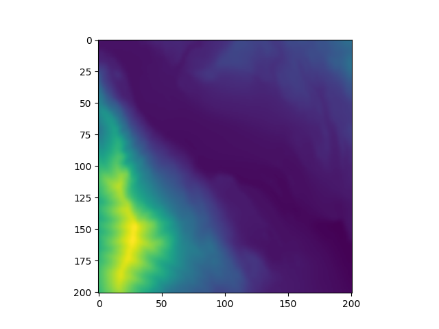
Get x, y and z (topography) arrays

x, y, z = res.x, res.y, res.z
fig, axe = plt.subplots()
axe.imshow(z)

<matplotlib.image.AxesImage object at 0x7ad0adf1bed0>

You can also display the topography with the pytopomap package is installed along with tilupy).

pytopomap.plot.plot_topo(z, x, y)

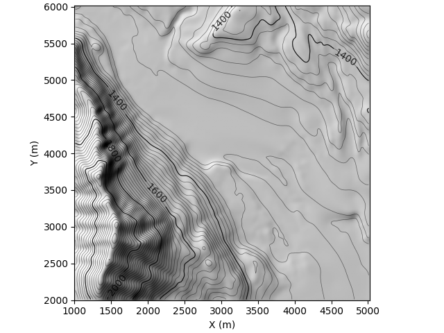
<Axes: xlabel='X (m)', ylabel='Y (m)'>

Simulation results get be obtained with the ‘get_output’ method and the name of the Result type. A ‘Result’ instance has several attributes describing it (e.g. name, unit, time, …), the raw data is loaded in the attribute ‘d’ in a ‘numpy.ndarray’.

For instance to get the thickness recorded at different time steps:

h_res = res.get_output("h")
print(h_res.t)
plt.imshow(h_res.d[:, :, -1])  # Plot final thickness.

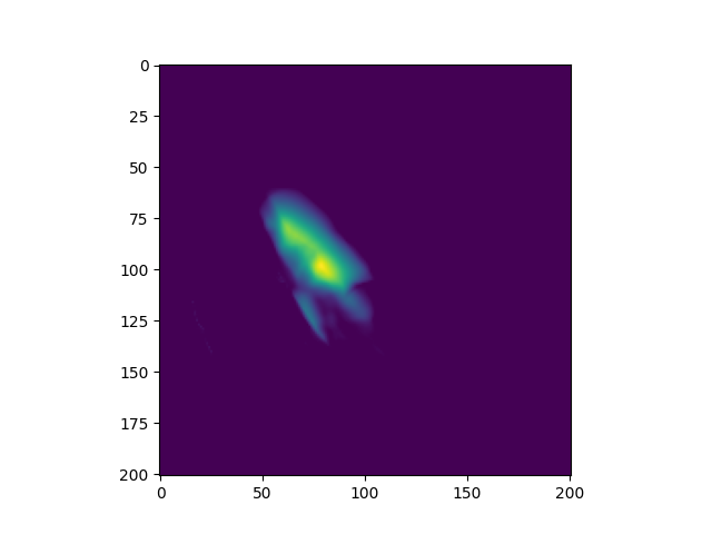
[  0.  10.  20.  30.  40.  50.  60.  70.  80.  90. 100.]

<matplotlib.image.AxesImage object at 0x7ad0adefd810>

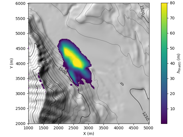
The final thickness can also be derived more directly with h_final. It can be plotted on the topography with built-in functions returning the axe where the plot was created. Note that an already existing axe instance can be used with the ax parameter of the plot method.

h_final = res.get_output("h_final")
axe = h_final.plot()

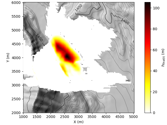
[WARNING] h_final not found with _read_from_file for shaltop, use get_spatial_stat

Due to numerical dispersion, a large area is covered with a very thin layer of materials at the end of the simulation, which is not physically relevant. This can be removed from plots by imposing a minimum value. More generally, is the case of 2D data (tilupy.read.TEMPORAL_DATA_2D and tilupy.read.STATIC_DATA_2D), plots can be customized with parameters passed on to pytopomap.plot.plot_data_on_topo(), for instance:

# Parameters for topography
topo_kwargs = dict(
    contour_step=50,  # Interval between thin contour lines
    step_contour_bold=250,  # Interval between bold contour lines
)
# parameters passed on to pytopomap.plot.plot_data_on_topo
kwargs = dict(
    vmin=0.2,  # Minimum value to be displayed
    vmax=80,  # Maximum value to be displayed
    cmap="viridis",  # Colormap setting
    topo_kwargs=topo_kwargs,
)

Here, the following call to the plot method is equivalent to pytopomap.plot.plot_data_on_topo(res.x, res.y, res.z, h_final.d, **kwargs)

axe = h_final.plot(**kwargs)

Sequential colormaps can also be easily created.

kwargs = dict(
    cmap_intervals=[0.5, 2, 10, 25, 50, 75, 100],
    cmap="viridis",
    topo_kwargs=topo_kwargs,
)
h_final.plot(**kwargs)

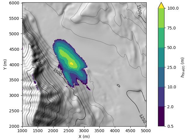
<Axes: xlabel='X (m)', ylabel='Y (m)'>