Plot front position over time.

This section shows how to use show_fronts_over_time function to plot front position depending on time.

For each case, we will use an initial water depth \(h_0 = 20m\). For Mangeney’s method, we use a slope of \(\theta = 30°\) and a friction angle of \(\delta = 25°\). For Stoker’s method, we use a domain depth of \(h_r = 1m\):

Implementation

from tilupy.analytic_sol import Front_result

import numpy as np

A = Front_result(h0=20)

---

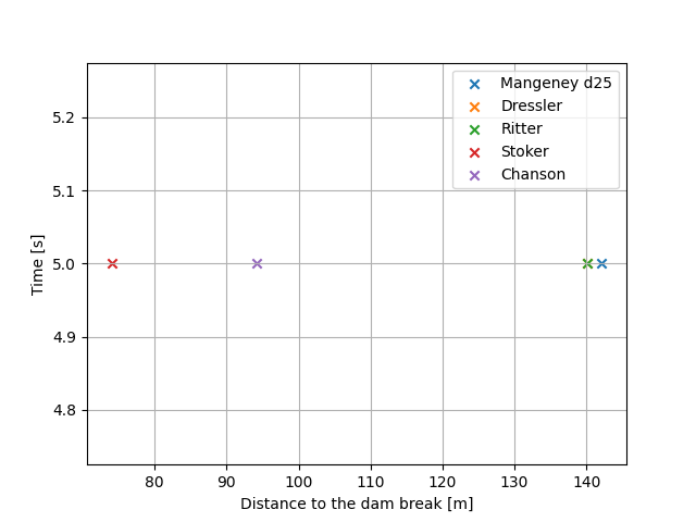
Case 1: computing only for \(t = 5s\).

t = 5

A.xf_mangeney(t, delta=25, theta=30)
A.xf_dressler(t)
A.xf_ritter(t)
A.xf_stoker(t, hr=1)
A.xf_chanson(t, f=0.05)

A.show_fronts_over_time()

---

Case 2: computing for \(t = {1, 5, 10, 15, 20}s\).

T = [1, 10, 15, 20]  # t = 5 already compute

for t in T:
    A.xf_mangeney(t, delta=25, theta=30)
    A.xf_dressler(t)
    A.xf_ritter(t)
    A.xf_stoker(t, hr=1)
    A.xf_chanson(t, f=0.05)

A.show_fronts_over_time()

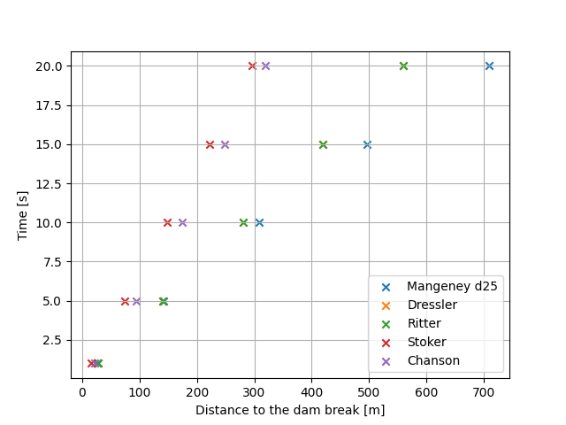
Ritter and Dressler’s solutions are the same.

---

Case 3: computing for \(t \in [0, 20]\).

T = np.linspace(0, 20, 100)  # t = 5 already compute

A = Front_result(h0=20)  # Reset values

for t in T:
    A.xf_mangeney(t, delta=25, theta=30)
    A.xf_dressler(t)
    A.xf_ritter(t)
    A.xf_stoker(t, hr=1)
    A.xf_chanson(t, f=0.05)

A.show_fronts_over_time()

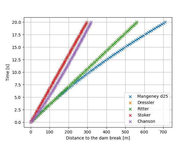
Ritter and Dressler’s solutions are the same.